Basalt

XML Input File

The basename for this file is basalt_circle.xml. The file can be run using this command:

microstructpy --demo=basalt_circle.xml

The full text of the file is:

<?xml version="1.0" encoding="UTF-8"?>
<input>
    <material>
        <name> Plagioclase </name>
        <fraction>
            <dist_type> norm </dist_type>
            <loc> 45.2 </loc>
            <scale> 0.2 </scale>
        </fraction>
        <size>
            <dist_type> cdf </dist_type>
            <filename> aphanitic_cdf.csv </filename>
        </size>
        <color> #BDBDBD </color>
    </material>

    <material>
        <name> Olivine </name>
        <shape> ellipse </shape>
        <fraction>
            <dist_type> norm </dist_type>
            <loc> 19.1 </loc>
            <scale> 0.2 </scale>
        </fraction>
        <size>
            <dist_type> cdf </dist_type>
            <filename> aphanitic_cdf.csv </filename>
        </size>
        <aspect_ratio>
            <dist_type> uniform </dist_type>
            <loc> 1.0 </loc>
            <scale> 2.0 </scale>
        </aspect_ratio>
        <angle_deg>
            <dist_type> uniform </dist_type>
            <loc> -90 </loc>
            <scale> 180 </scale>
        </angle_deg>
        <color> #99BA73 </color>
    </material>

    <material>
        <name> Diopside </name>
        <fraction>
            <dist_type> norm </dist_type>
            <loc> 13.2 </loc>
            <scale> 0.2 </scale>
        </fraction>
        <size>
            <dist_type> cdf </dist_type>
            <filename> aphanitic_cdf.csv </filename>
        </size>
        <color> #709642 </color>
    </material>

    <material>
        <name> Hypersthene </name>
        <fraction>
            <dist_type> norm </dist_type>
            <loc> 16.6 </loc>
            <scale> 0.2 </scale>
        </fraction>
        <size>
            <dist_type> cdf </dist_type>
            <filename> aphanitic_cdf.csv </filename>
        </size>
        <color> #876E59 </color>
    </material>

    <material>
        <name> Magnetite </name>
        <fraction>
            <dist_type> norm </dist_type>
            <loc> 3.35 </loc>
            <scale> 0.2 </scale>
        </fraction>
        <size>
            <dist_type> cdf </dist_type>
            <filename> aphanitic_cdf.csv </filename>
        </size>
        <color> #6E6E6E </color>
    </material>

    <material>
        <name> Chromite </name>
        <fraction>
            <dist_type> norm </dist_type>
            <loc> 0.65 </loc>
            <scale> 0.2 </scale>
        </fraction>
        <size>
            <dist_type> cdf </dist_type>
            <filename> aphanitic_cdf.csv </filename>\
        </size>
        <color> #545454 </color>
    </material>

    <material>
        <name> Ilmenite </name>
        <fraction>
            <dist_type> norm </dist_type>
            <loc> 0.65 </loc>
            <scale> 0.2 </scale>
        </fraction>
        <size>
            <dist_type> cdf </dist_type>
            <filename> aphanitic_cdf.csv </filename>
        </size>
        <color> #6B6B6B </color>
    </material>

    <material>
        <name> Apatite </name>
        <fraction>
            <dist_type> norm </dist_type>
            <loc> 3.35 </loc>
            <scale> 0.2 </scale>
        </fraction>

        <size>
            <dist_type> cdf </dist_type>
            <filename> aphanitic_cdf.csv </filename>
        </size>
        <color> #ABA687 </color>
    </material>

    <domain>
        <shape> circle </shape>
        <diameter> 6 </diameter>
    </domain>

    <settings>
        <directory> basalt_circle </directory>
        <filetypes>
            <seeds_plot> png </seeds_plot>
            <poly_plot> png </poly_plot>
            <tri_plot> png </tri_plot>
            <verify_plot> png </verify_plot>
        </filetypes>

        <plot_axes> False </plot_axes>
        <verbose> True </verbose>
        <verify> True </verify>

        <mesh_max_edge_length> 0.01 </mesh_max_edge_length>
        <mesh_min_angle> 20 </mesh_min_angle>
        <mesh_max_volume> 0.05 </mesh_max_volume>

        <seeds_kwargs>
            <linewidths> 0.2 </linewidths>
        </seeds_kwargs>
        <poly_kwargs>
            <linewidths> 0.2 </linewidths>
        </poly_kwargs>
        <tri_kwargs>
            <linewidths> 0.1 </linewidths>
        </tri_kwargs>
    </settings>
</input>

Material 1 - Plagioclase

Plagioclase composes approximately 45% of this basalt sample. It is an aphanitic component, meaning fine-grained, and follows a custom size distribution.

Material 2 - Olivine

Olivine composes approximately 19% of this basalt sample and is also an aphanitic component. The orientation of the olivine crystals is uniform random, with the aspect ratio varying from 1 to 3 uniformly.

Materials 3-8

Diopside, hypersthene, magnetite, chromite, ilmenite, and apatie compose approximately 36% of this basalt sample. They are aphanitic components and follow a custom size distribution, but are generally circular in shape.

Domain Geometry

These materials fill a circular domain with a diameter of 6 mm.

Settings

The function will output plots of the microstructure process and those plots are saved as PNGs. They are saved in a folder named basalt_circle, in the current directory (i.e ./basalt_circle).

The axes are turned off in these plots, creating PNG files with minimal whitespace.

Mesh controls are introducted to increase grid resolution, particularly at the grain boundaries.

Output Files

The three plots that this file generates are the seeding, the polygon mesh, and the triangular mesh. These three plots are shown in Fig. 10 - Fig. 12.

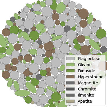
Fig. 10 Basalt example - seed geometries

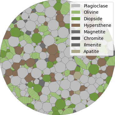
Fig. 11 Basalt example - polygonal mesh

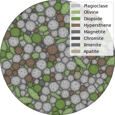
Fig. 12 Basalt example - triangular mesh

With the <verification> flag set to True, verification plots are generated by MicroStructPy. The grain size distribution comparison is given in Fig. 13.

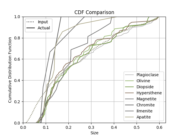
Fig. 13 Basalt example - input and output crystal size distributions (CSDs).

Comparing the input and output distributions, it is clear that this microstructure is not statistically representative. A larger diameter for the domain would contain more grains of olivine, which would add more fidelity to the size CDF curve.