6. Culmination
6.1. XML Input File
The basename for this file is intro_6_culmination.xml.
The file can be run using this command:
microstructpy --demo=intro_6_culmination.xml
The full text of the file is:
<?xml version="1.0" encoding="UTF-8"?>
<input>
    <material>
        <material_type> matrix </material_type>
        <fraction> 2 </fraction>

        <shape> circle </shape>
        <size>
            <dist_type> uniform </dist_type>
            <loc> 0 </loc>
            <scale> 1.5 </scale>
        </size>
        <color> pink </color>
    </material>

    <material>
        <fraction> 1 </fraction>
        <shape> ellipse </shape>
        <size>
            <dist_type> triang </dist_type>
            <loc> 0 </loc>
            <scale> 2 </scale>
            <c> 1 </c>
        </size>
        <aspect_ratio>
            <dist_type> uniform </dist_type>
            <loc> 1 </loc>
            <scale> 2 </scale>
        </aspect_ratio>
        <angle_deg>
            <dist_type> uniform </dist_type>
            <loc> -10 </loc>
            <scale> 20 </scale>
        </angle_deg>
        <color> lime </color>
    </material>

    <domain>
        <shape> square </shape>
        <side_length> 20 </side_length>
        <corner> (0, 0) </corner>
    </domain>

    <settings>
        <filetypes>
            <seeds_plot> png </seeds_plot>
            <poly_plot> png, pdf </poly_plot>
            <tri_plot> png </tri_plot>
            <tri_plot> eps </tri_plot>
            <tri_plot> pdf </tri_plot>
        </filetypes>

        <directory> intro_6_culmination </directory>
        <verbose> True </verbose>

        <mesh_min_angle> 25 </mesh_min_angle>
        <mesh_max_volume> 1 </mesh_max_volume>
        <mesh_max_edge_length> 0.1 </mesh_max_edge_length>

        <seeds_kwargs>
            <alpha> 0.5 </alpha>
            <edgecolors> none </edgecolors>
        </seeds_kwargs>

        <poly_kwargs>
            <linewidth> 3 </linewidth>
            <edgecolors> #A4058F </edgecolors>
        </poly_kwargs>

        <tri_kwargs>
            <linewidth> 0.2 </linewidth>
            <edgecolor> navy </edgecolor>
        </tri_kwargs>

        <plot_axes> False </plot_axes>
    </settings>
</input>
6.2. Materials
There are two materials, in a 2:1 ratio based on volume. The first is a pink matrix, which is represented with small circles.
The second material consists of lime green elliptical inclusions with size ranging from 0 to 2 and aspect ratio ranging from 1 to 3. Note that the size is defined as the diameter of a circle with equivalent area. The orientation angle of the inclusions are uniformly distributed between -10 and +10 degrees, relative to the +x axis.
6.3. Domain Geometry
These two materials fill a square domain. The bottom-left corner of the rectangle is the origin, which puts the rectangle in the first quadrant. The side length is 20, which is 10x the size of the inclusions.
6.4. Settings
PNG files of each step in the process will be output, as well as the
intermediate text files.
They are saved in a folder named intro_5_plotting, in the current directory
(i.e ./intro_5_plotting).
PDF files of the poly and tri mesh are also generated, plus an EPS file for the
tri mesh.
The seeds are plotted with transparency to show the overlap between them. The poly mesh is plotted with thick purple edges and the tri mesh is plotted with thin navy edges.
In all of the plots, the axes are toggles off, creating image files with minimal borders.
The minimum interior angle of the elements is 25 degrees, ensuring lower aspect ratios compared to the first example. The maximum area of the elements is also limited to 1, which populates the matrix with smaller elements. Finally, The maximum edge length of elements at interfaces is set to 0.1, which increasing the mesh density surrounding the inclusions and at the boundary of the domain.
Note that the edge length control is currently unavailable in 3D.
6.5. Output Files
The three plots that this file generates are the seeding, the polygon mesh, and the triangular mesh. These three plots are shown in Fig. 6.1 - Fig. 6.3.
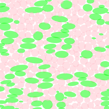
Fig. 6.1 Introduction 6 - seed geometries.
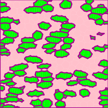
Fig. 6.2 Introduction 6 - polygonal mesh.
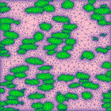
Fig. 6.3 Introduction 6 - triangular mesh.